From Spin to Signal: The physics behind the 1.42 GHz Hydrogen Line

The 21cm hydrogen line was first theoretically predicted in 1944 by Dutch astronomer Hendrik van de Hulst. Its initial detection seven years later marked the birth of 21cm astronomy. This discovery was made simultaneously in 1951 by Harold Ewen and Edward Purcell at Harvard University, who built a revolutionary horn antenna to capture the signal from our galaxy.

This discovery opened the cosmos to spectral line radio astronomy. Since then, measuring the Doppler shift of this specific frequency has become a staple project for aspiring radio amateurs. By comparing the observed frequency from observed Hydrogen clouds to the known laboratory value of $1420\;405\;751.768 \pm 0.002 \; \mathrm{Hz}$¹, the precise radial velocities can be calculated. But why is this radiation emitted at this exact frequency?

In this article, I will derive the hyperfine transition of the hydrogen ground state resulting in this emission using the machinery of quantum mechanics and electrodynamics and attempt to present it as clearly as possible, aimed at the level of a motivated undergraduate who has taken introductory courses in these fields. This work follows the outline established by David Griffiths in his 1982 derivation².

Setup

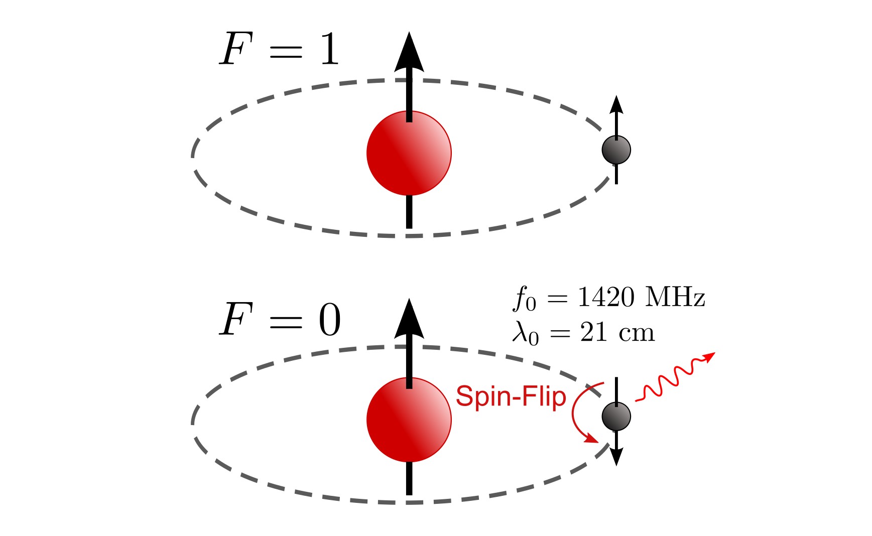
The system of the electron “orbiting” the proton can be thought of as two magnetic dipoles with a certain relative orientation (parallel or anti-parallel). The proton itself has an intrinsic magnetic moment arising from its spin, and this generates a magnetic field that extends into the region of the electron. The electron, carrying both charge and spin, also possesses a magnetic moment.

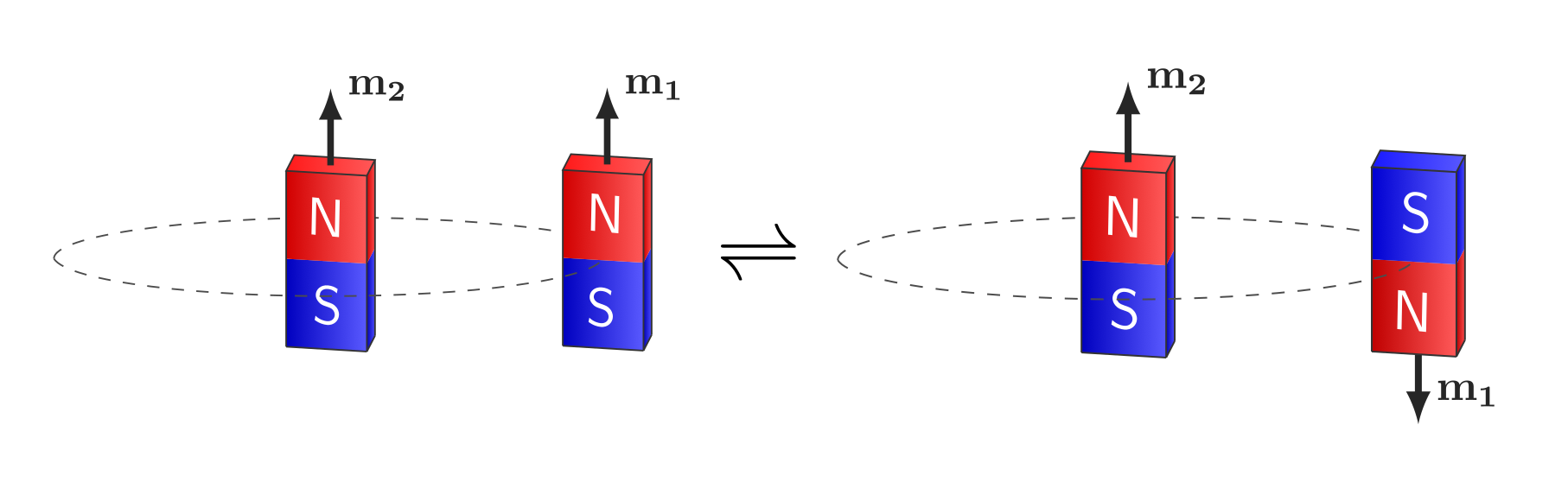Transition between parallel and anti-parallel orientations of the electron and proton in Hydrogen, represented by bar magnets.

It can be shown that the anti-parallel configuration has lower energy.² Intuitively, this corresponds to opposite poles aligning, where the dipoles attract more strongly, in contrast to the parallel configuration where like poles oppose each other and the energy of the system is higher.

Derivation

The interaction Hamiltonian for a magnetic moment in a field is $H_{\text{int}} = -\mathbf{m} \cdot \mathbf{B}$. In the hydrogen atom there are two such moments, the electron’s magnetic moment $\mathbf{m_1}$ and the proton’s magnetic moment $\mathbf{m_2}$. The magnetic field $B$ acting on the electron arises from $\mathbf{m_2}$ and is given by²

\[\mathbf{B}(\mathbf{r}) = \frac{\mu_0}{4\pi} \frac{1}{r^3} \left[3(\mathbf{m}_2 \cdot \hat{\mathbf{r}})\hat{\mathbf{r}} - \mathbf{m}_2\right] + \frac{2\mu_0}{3}\mathbf{m}_2 \, \delta^3(\mathbf{r})\]

Thus, the dipole-dipole interaction Hamiltonian is:

\[H_{\text{int}} = \underbrace{-\frac{\mu_0}{4\pi r^3} \left[3 (\mathbf{m}_1 \cdot \hat{\mathbf{r}}) (\mathbf{m}_2 \cdot \hat{\mathbf{r}}) - \mathbf{m}_1 \cdot \mathbf{m}_2\right] }_{H_{\text{dipole}}} - \underbrace{\frac{2\mu_0}{3} (\mathbf{m}_1 \cdot \mathbf{m}_2) \, \delta^3(\mathbf{r})}_{H_{\text{contact}}}\]

The ground-state wavefunction of the hydrogen electron can be written as a product of the spatial and spin parts

\[\Psi(\mathbf{r}) = \psi_{100} \; \ket{\chi},\quad \psi_{100}(\mathbf{r}) = \frac{1}{\sqrt{\pi a^3}} e^{-r/a}\]

with $a$ as the Bohr radius and $\ket{\chi}$ as the spin state.

First order perturbation theory

The full Hamiltonian is decomposed into the unperturbed part and the hyperfine interaction: $H = H_0 + H_{\text{int}}$. The unperturbed part in this example represents the hydrogen atom only under influence of the Coulomb law, $H_0 = -\frac{\hbar^2}{2m} \nabla^2 - \frac{e^2}{4\pi \epsilon_0} \frac{1}{r}$. The first-order energy correction is given by the expectation value of the perturbation Hamiltonian:

\[\begin{align*} E' &= \bra{\Psi} H_{\text{int}} \ket{\Psi} \\ &= \bra{\Psi} H_{\text{dipole}} \ket{\Psi} + \bra{\Psi} H_{\text{contact}} \ket{\Psi} \end{align*}\]

The dipole term $H_{\text{dipole}}$ does not contribute in the ground state because the hydrogen $1s$ wavefunction is spherically symmetric. The magnetic dipole field,

\[\mathbf{B}(\mathbf{r}) \;\propto\; \frac{1}{r^3}\left(3(\hat{\mathbf{r}}\cdot \mathbf{m_2})\hat{\mathbf{r}} - \mathbf{m_2}\right),\]

when integrated over the entire sphere, goes to zero.³

\[\bra{\Psi} H_{\text{dipole}} \ket{\Psi} = 0 .\]

Now we only have to deal with the dirac-delta pulse at the origin. Substituting the magnetic moments,

\[\begin{align*} \bra{\Psi} H_{\text{contact}} \ket{\Psi} &= \bra{\Psi} \frac{-2 \mu_0}{3} \, (\mathbf{m_1} \cdot \mathbf{m_2}) \, \delta^3(\mathbf{r}) \ket{\Psi} \end{align*}\]

This leaves only the contact term $H_\text{contact}$, separating spatial and spin parts in the state $\ket{\Psi} = \ket{\psi}\ket{\chi}$

\[\begin{align*} &= \frac{-2 \mu_0}{3} \bra{\chi} \mathbf{m_1} \cdot \mathbf{m_2} \ket{\chi} \bra{\Psi} \delta^3(\mathbf{r}) \ket{\Psi} \\ &= \frac{-2 \mu_0}{3} \braket{\mathbf{m_1} \cdot \mathbf{m_2}} \cdot \int |\Psi(r)|^2 \delta^3(\mathbf{r}) d\tau \end{align*}\]

Use the dirac delta property $\int f(\mathbf{r}) \delta^3(\mathbf{r}) d\tau = f(0)$,

\[\begin{align*} &= \frac{-2 \mu_0}{3} \braket{\mathbf{m_1} \cdot \mathbf{m_2}} \cdot |\Psi(0)|^2 \end{align*}\]

The probability density of the wavefunction is $\lvert \Psi(r) \rvert^2 = \frac{1}{\pi a^3} e^{-2r/a} \;$ then clearly $\lvert \Psi(0) \rvert^2 = 1/ \pi a^3$

\[\begin{align*} &= \frac{-2 \mu_0}{3 \pi a^3} \braket{\mathbf{m_1} \cdot \mathbf{m_2}} \end{align*}\]

The magnetic moments $\mathbf{m_1}$ and $\mathbf{m_2}$ of respectively the proton and electron are proportional to their spin with gyromagnetic constants $\gamma_p$ and $\gamma_e$ expressed in units of frequency. These are more commonly expressed in terms of the Landé $g$-factors and particle masses as

\[\begin{align*} \mathbf{m_1} = \gamma_p \, I = \frac{g_p\, e}{2 m_p}\, I, \quad \mathbf{m_2} = - \gamma_e \, S = - \frac{g_e\, e}{2 m_e}\, S \end{align*}\]

The minus sign for the electron reflects its negative charge, so its magnetic moment points opposite to its spin. So now

\[\begin{align*} E' &= \frac{-2 \mu_0}{3 \pi a^3} \braket{\mathbf{m_1} \cdot \mathbf{m_2}} \\ &= \frac{-2 \mu_0}{3 \pi a^3} \frac{g_p \, e}{2m_p} \, \left(-\frac{g_e \, e}{2m_e}\right) \braket{I \cdot S} \\ &= \frac{\mu_0\,e^2}{6 \pi a^3} \frac{g_p g_e}{m_p m_e} \braket{I \cdot S} \end{align*}\]

Now what is the expectation value of $I \cdot S$ ?

Consider the total angular momentum $F \equiv I + S$, then

\[\begin{align*} F^2 &= (I + S)^2 = I^2 + S^2 + 2 I \cdot S \\ &\Leftrightarrow I \cdot S = \frac{1}{2}\left(F^2 - I^2 - S^2 \right) \\ &\Leftrightarrow \braket{I \cdot S} = \frac{1}{2}\left(\braket{F}^2 - \braket{I}^2 - \braket{S}^2 \right) \end{align*}\]

As we are interested in the transition from spin up ($m_s = 1/2$) to spin down ($m_s = -1/2$) while keeping the spin of the proton constant ($m_I = 1/2$), the total spin F changes accordingly between the triplet ($F = 1$) and singlet ($F = 0$) states.

We can use an important result of the algebraic theory of spin⁴, $S^2 \ket{s\;m} = s(s+1)\hbar^2 \ket{s\;m}$, to find the values that $S^2$, $I^2$ and $F^2$ may take on.

Triplet state (F = 1)

For the triplet state, we have $m_s = 1/2$, $m_I = 1/2$ and $F = 1$ then

\[\begin{align*} \braket{S^2} &= \frac{1}{2}\left(1+\frac{1}{2}\right) \hbar^2 = \frac{3}{4} \hbar^2\\ \braket{I^2} &= \frac{1}{2}\left(1+\frac{1}{2}\right) \hbar^2 = \frac{3}{4} \hbar^2\\ \braket{F^2} &= 1\left(1+1\right) \hbar^2 = 2 \hbar^2\\ \end{align*}\]

so now the expectation value takes on,

\[\begin{align*} \braket{I \cdot S} &= \frac{1}{2}\left(\braket{F}^2 - \braket{I}^2 - \braket{S}^2 \right) \\ &= \frac{1}{2}\left(2\hbar^2 - \frac{3}{4}\hbar^2 - \frac{3}{4}\hbar^2\right) \\ &= \frac{1}{4}\hbar^2 \end{align*}\]

Singlet state (F = 0)

For the singlet state, we have $m_s = -1/2$, $m_I = 1/2$ and $F = 0$ then

\[\begin{align*} \braket{S^2} &= \frac{1}{2}\left(1+\frac{1}{2}\right) \hbar^2 = \frac{3}{4} \hbar^2\\ \braket{I^2} &= \frac{1}{2}\left(1+\frac{1}{2}\right) \hbar^2 = \frac{3}{4} \hbar^2\\ \braket{F^2} &= 0\left(1+0\right) \hbar^2 = 0 \hbar^2\\ \end{align*}\]

so now the expectation value takes on,

\[\begin{align*} \braket{I \cdot S} &= \frac{1}{2}\left(\braket{F}^2 - \braket{I}^2 - \braket{S}^2 \right) \\ &= \frac{1}{2}\left(0 - \frac{3}{4}\hbar^2 - \frac{3}{4}\hbar^2\right) \\ &= -\frac{3}{4}\hbar^2 \end{align*}\]

and in conclusion,

\[\braket{I \cdot S} = \begin{cases} \frac{1}{4}\hbar^2 &(\mathrm{triplet})\\ -\frac{3}{4}\hbar^2 &(\mathrm{singlet}) \end{cases}\]

Note: we cannot consider the $S$ and $I$ $z$-components seperately due to spin-spin coupling between the proton and electron, therefore we used the total angular momentum $F$.

Energies

To find the energies of each state, we can substitute the expectation value as

\[\begin{align*} E' &= \frac{\mu_0\,e^2}{6 \pi a^3} \frac{g_p g_e}{m_p m_e} \braket{I \cdot S} \\ &= \frac{\mu_0\,e^2}{6 \pi a^3} \frac{g_p g_e}{m_p m_e} \begin{cases} \frac{1}{4}\hbar^2 &(\mathrm{triplet})\\ -\frac{3}{4}\hbar^2 &(\mathrm{singlet}) \end{cases} \end{align*}\]

Finding the energy transition between these states is now trivially easy by taking the difference,

\[\begin{align*} \Delta E' &= \frac{\mu_0\,e^2}{6 \pi a^3} \frac{g_p g_e}{m_p m_e} \left(- \frac{3}{4} - \frac{1}{4} \right)\hbar^2 \\ &= -\frac{\mu_0 e^2 \hbar^2}{6 \pi a^3} \frac{g_p g_e}{m_p m_e} \end{align*}\]

Now we have an expression in which all parameters can be determined experimentally. By substituting the known values of the physical constants:⁵

• $ m_e = 9.109\;383\;713 \times 10^{-31} \, \text{kg}$
• $ m_p = 1.672\;621\;925 \times 10^{-27} \, \text{kg}$
• $ a = 5.291\;772\;105 \times 10^{-11} \, \text{m} $
• $ \hbar = 1.054\;571\;817 \times 10^{-34} \, \text{J s}$
• $ e = 1.602\;176\;634 \times 10^{-19} \, \text{C}$
• $ g_e = -2.002\;319\;304$
• $ g_p = 5.585\;694\;6893$

\[\begin{align*} \Delta E' &= -\frac{\mu_0 \hbar^2 e^2}{6 \pi a^3} \frac{g_p g_e}{m_e m_p} \\ &\approx 9.427\,622\,815 \times 10^{-25} \text{J} \end{align*}\]

Using the Planck relation $E = hf$, with Planck constant $h = 6.626\;070\;15 \times 10^{-34} \, \text{J/Hz}$

\[f = \frac{\Delta E'}{h} \approx 1422\,807\,577.0611868 \, \text{Hz} \approx 1.42281 \, \text{GHz}\]

Or expressed as a wavelength with $\lambda = \frac{v}{f}$ and speed of light $c$,

\[\lambda = \frac{c}{f} \approx 21.0705 \, \text{cm}\]

These values are in close agreement with the observed laboratory value¹, the small error is due to taking only the first order perturbation approximation neglecting higher-order QED and nuclear corrections.

Sources

1. Peters, H. E., et al. “Measurement of the Unperturbed Hydrogen Hyperfine Transition Frequency.” IEEE Transactions on Instrumentation and Measurement, vol. IM-19, no. 4, Nov. 1970, pp. 342-48. IEEE Xplore, doi:10.1109/TIM.1970.4313902. ↩︎ ↩︎²

2. Griffiths, D. J. “Hyperfine Splitting in the Ground State of Hydrogen.” American Journal of Physics, vol. 50, no. 8, Aug. 1982, p. 698. AIP Publishing, doi:10.1119/1.12733. ↩︎ ↩︎² ↩︎³

3. David J. Griffiths, Introduction to Quantum Mechanics, 3rd ed., Exercise 7.31 ↩︎

4. David J. Griffiths, Introduction to Quantum Mechanics, 3rd ed., Eq. 4.135 ↩︎

5. National Institute of Standards and Technology (NIST), CODATA Recommended Values of the Fundamental Physical Constants: 2018–2022, https://physics.nist.gov/cuu/Constants/index.html. ↩︎